Humanoid Arm Manipulation using Deep Reinforcement Learning
This work is a showcase of my bachelor’s thesis at CNRS-AIST Joint Robotics Laboratory on Humanoid Arm Manipulation using Deep Reinforcement Learning.
This is a work that marks the first step taken in working towards the locomotion of a humanoid in contact-rich environments, where manipulation is required to assist the walking of the robot.
About the Algorithm & Network:
Proximal Policy Optimization (PPO)
Proximal Policy Optimization is a prominent policy gradient algorithm in the field of reinforcement learning in robotics. Some of the key features of this algorithm are:
- Objective Function: PPO modifies the policy gradient objective to limit the size of the policy update at each step, which addresses the issue of having excessively large policy updates that can lead to performance degradation. It uses a clipped surrogate objective function, which prevents the policy from changing too drastically, aiding in stable learning.
Clipping Mechanism: The core idea in PPO is to clip the probability ratio between the old policy (before update) and the new policy (after update), thus bounding the updates to the policy. This clipping mechanism keeps the update within a range defined by a hyperparameter, ε (epsilon).
The objective function of PPO looks to maximize the clipped surrogate objective: \[L^{CLIP}(θ)=E_t[min(r_t(θ)A_t,clip(r_t(θ),1−ϵ,1+ϵ)A_t)]\]
Here \(r_t(θ)\) signifies the ratio of the probabilities of new policy to old policy
\(A_t\) is the advantage estimator at time t.
- Advantage Estimation: PPO uses Generalized Advantage Estimation (GAE) for estimating the advantage values for determining the direction and magnitude of the policy update.
Implemented in Actor-Critic Style Neural Network
\(n_O\): number of observations
\(n_A\): number of actions
Actor network dimensions: \(n_O×256×256×256×n_A\)
Critic network dimensions: \(n_O×256×256×256×1\)
- Actor: The actor component is responsible for selecting actions. It is essentially a policy function that maps states to actions. The actor is typically represented as a parameterised function, often a neural network, whose parameters are adjusted to improve the policy based on feedback from the critic.
- Critic: The critic evaluates the actions taken by the actor by computing a value function. This value function can either be a state-value function \(V(s)\) (which estimates how good it is to be in a given state) or an action-value function \(Q(s,a)\) (which estimates the value of taking a certain action in a given state). The critic’s role is to estimate the error in the policy’s action predictions, which is used to update both the critic and the actor.
Temporal Difference Error: The TD error is given by: \(δ=r+γV(s^′)−V(s)\) Here \(r\) is the reward received when an agent in state \(s\) has taken an action \(a\). \(γ\) is the discount factor and \(V(s^′)\) is the value of next state \(s^′\), \(V(s)\) is the value of state \(s\).
The total positive term \(r+γV(s^′)\) is the estimate of total return after taking the action \(a\) in state \(s\) and then going to state \(s^′\) and thereon following the policy. The negative term \(V(s)\) is the value/estimate of total return while following the policy from state \(s\) of state.
A positive value of \(δ\) means the action \(a\) gave better than expected outcome whereas a negative value of \(δ\) means the outcome was worse than expected. Evidently, actions in the first case are favoured in the future while in the latter case are avoided by the policy.
- Policy Update: The actor takes care of the policy update using a gradient of a performance measure, in general the Temporal Difference error given by the critic. The policy is updated to maximise the expected return.
- Value Function Update: This is taken care of by the critic using the TD error. This error reflects how good the actor’s action was compared to the critic’s expectation.
Observations:
The nature of the observations is completely state-based, i.e. the prioperceptive data of the joint positions and velocities, the geometric center of the object, the actions the arm has performed etc. etc. Since the root link of the humanoid has been fixed during the simulations, the floating joint is not included in the observations.
These observations have been used accurately as is and also along with some noise introduced to enable robust training.
The part of the simulations comprised the 9 DoFs of the humanoid arm without including the joints of the fingers.
Actions:
The actions are generated from the observations input into the step function.
Action scaling and Action smoothening are performed right before sending the generated actions to the torques in the simulation to ensure smoothened actions are generated by the policy.
Torques:
Torques are generated with hit-and-trial based PD gains which are common to all the joints of the arm. The actions generated by the policy are passed on to formulate the torques using the gain values and these torques are fed into the simulator to showcase the results of the training done so far.
Simulation parameter tuning & URDF modification
The simulation environment in Isaac Gym requires tuning of certain parameters pertaining to the physics engine and others specific to the model of the robot imported into the simulation. Values such as joint armature, joint position limits, joint velocity limits etc. need to be tuned to ensure a stable simulation of the robot in the environment.
Also, the URDF model of the robot has been modified to include only the required joints of a single arm, omitting the legs and the left arm, leaving only the right arm of the robot functional. The robot is fixed at its base.
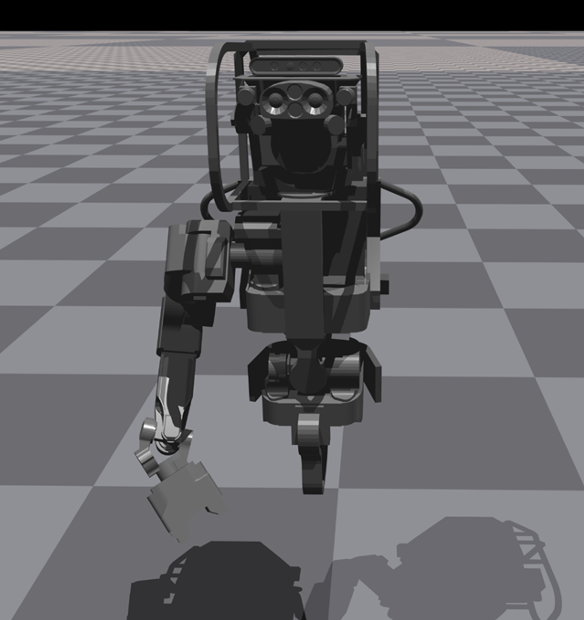
An illustration of the robot’s model in the Isaac Gym simulator
Tasks
The following tasks have been trained on the robot as steps towards working on object manipulation with the robot’s arm:
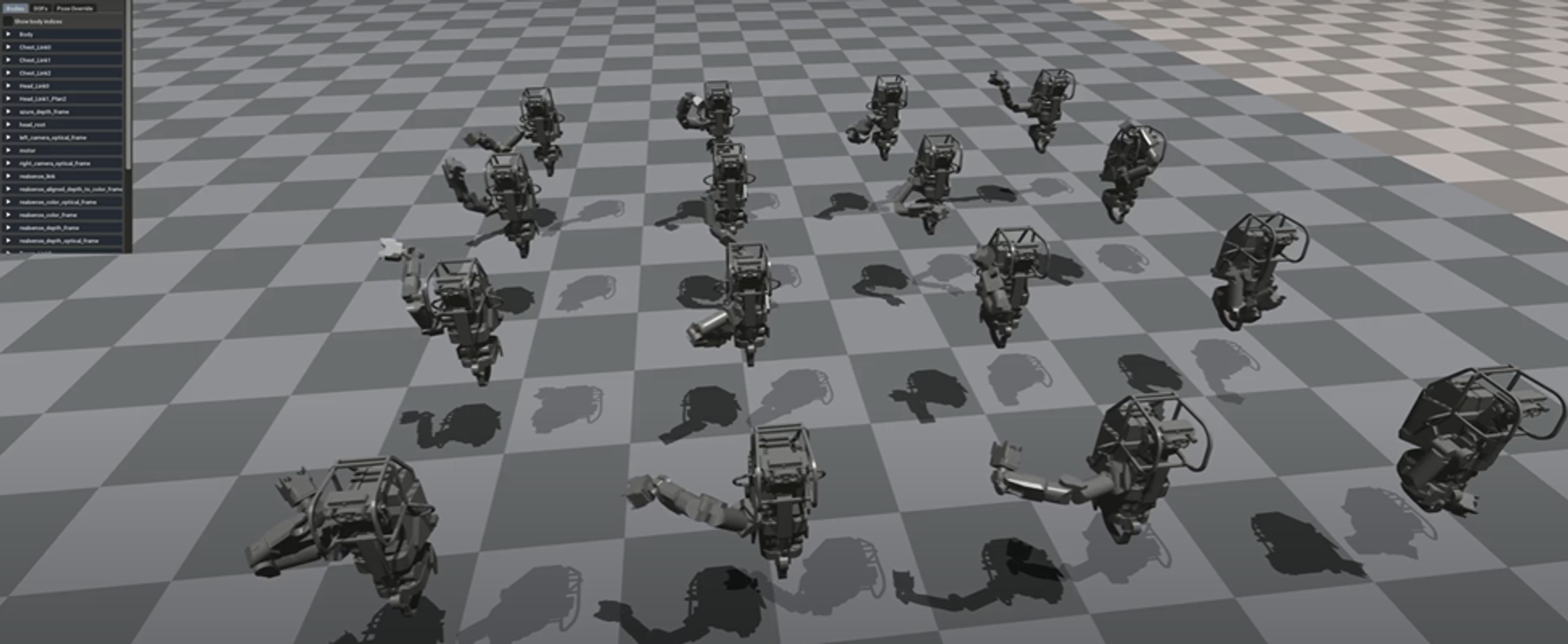
1. Reaching a fixed given 9-DoF pose from a random initial pose
The task involves spawning the robot in the 4096 environments in parallel in random 9-DoF poses for the arm and pushing them to reach a goal 9-DoF pose.
Observation Space: DoF positions and velocities
The observation space includes the 9-DoF poses and velocities of the robot. This implies that the policy/agent knows, at each control step, the DoF pose of the arm, which helps in calculating the error from the goal pose.
Reward: Minimise error dof pose, energy
The reward signal comprises the minimization of error of the DoF pose of the arm compared to the goal pose. It also pushes towards minimizing the energy (= torque × velocity) being spent by the joints in implementing the task.
An illustration from the simulator while testing the task 1.
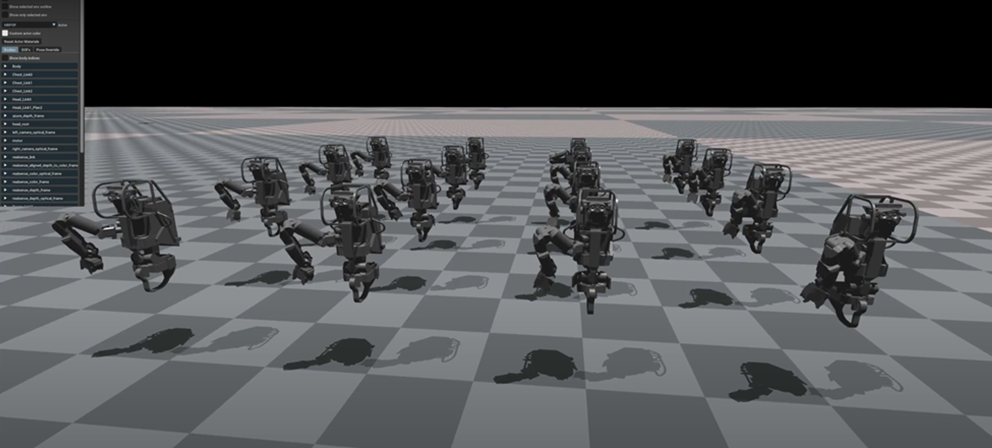
2. Reaching any given 9-DoF pose from a random initial pose
This is similar to the task discussed in 1, with the only difference in the goal DoF pose being different for each robot.
Observation Space: DoF positions and velocities, Goal DoF pose
Same as in 1., with an additional observation of the goal dof pose for each environment.
Reward: Minimise error dof pose, energy
Same as in 1.
An illustration from the simulator while testing the task 2.
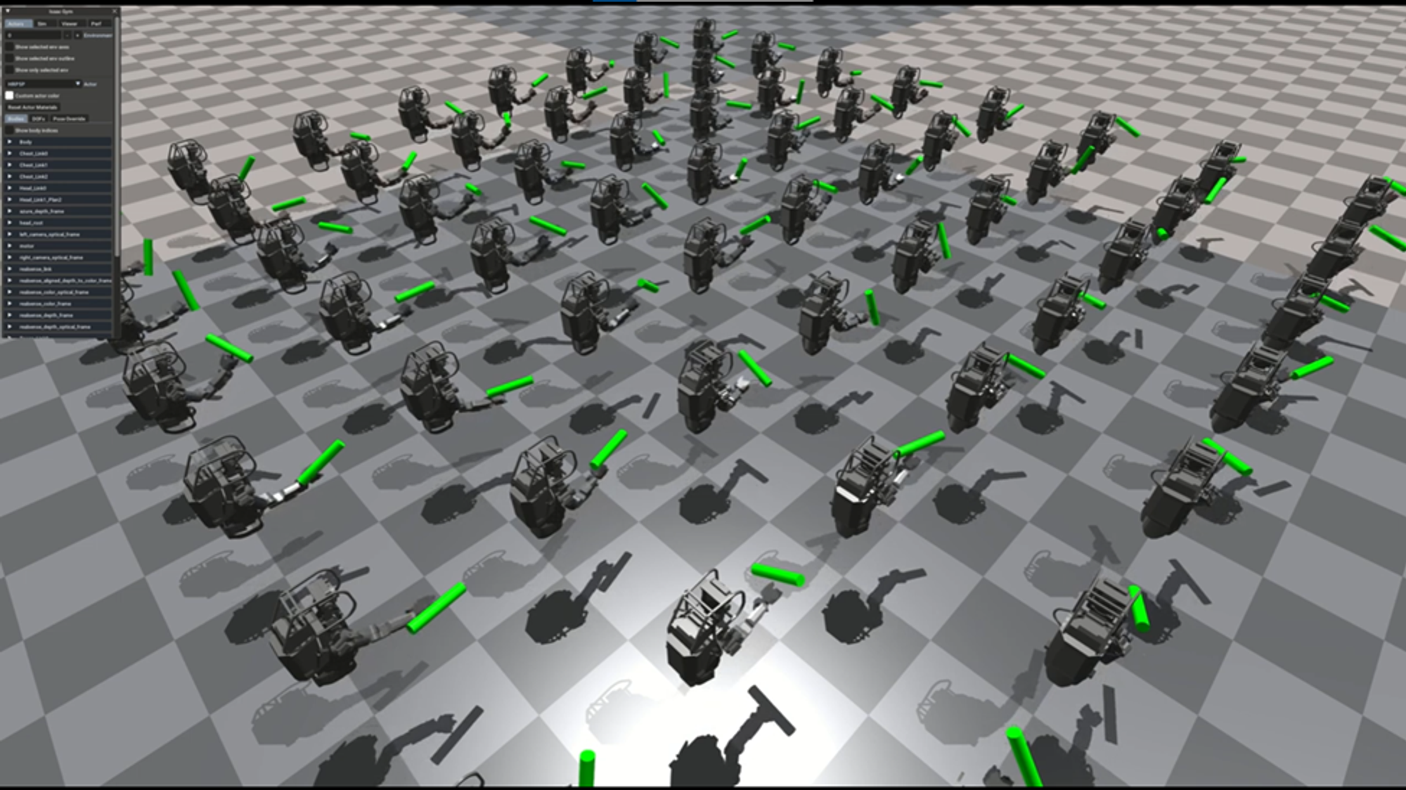
3. Reaching any given point in the Cartesian space from a random initial pose
This task involves training to reach a given 3D point in the Cartesian space around the robot in its environment. The arm is given a random initial pose in each of the parallel environments and the goal: 3D point is also a random point for each environment.
Observation Space: DoF positions and velocities, actions, goal position coordinates: 3 (x,y,z)
As compared to the observation spaces in the previous tasks, this task has a different observation space in terms of observing its own actions. The goal observed in this case is a 3D point in the Cartesian space for each robot.
Reward: Minimise error position, energy
The error minimization focuses on reducing the error of the end-effector 3D position and the observed goal position in the Cartesian space. Along with the error, the energy spent by the joints is minimized.
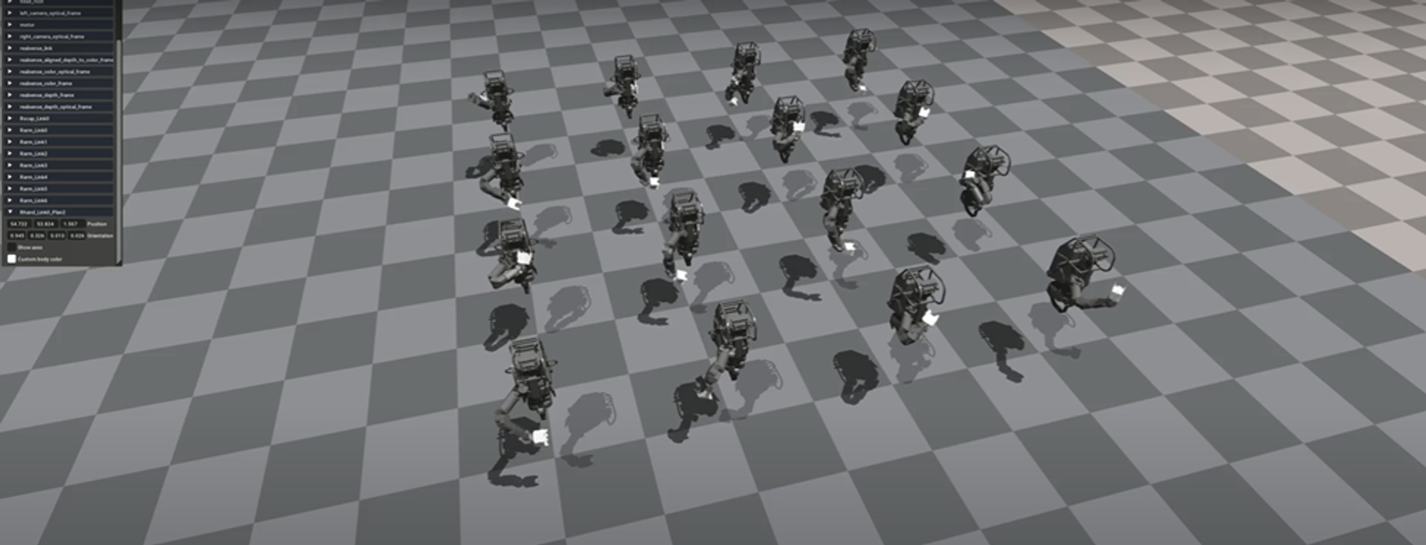
An illustration from the simulator while testing the task 3. The link white in color is the end-effector.
4. Reaching any given pose in the Cartesian space from a random initial pose
This task is quite similar to 3 with the difference being in trying to reduce the complete 6D pose (position + orientation) error of the end effector pose from the given goal pose
Observation Space: DoF positions and velocities, actions, goal pose coordinates: 3 position, 4 quaternion
Same in as 3. with a change in the size of the goal pose observed from 3D to 7: 3 for position, 4 for the quaternion representation of the orientation.
Reward: Minimise error pose, energy
The logic used in designing the rewards is the same as in 3.
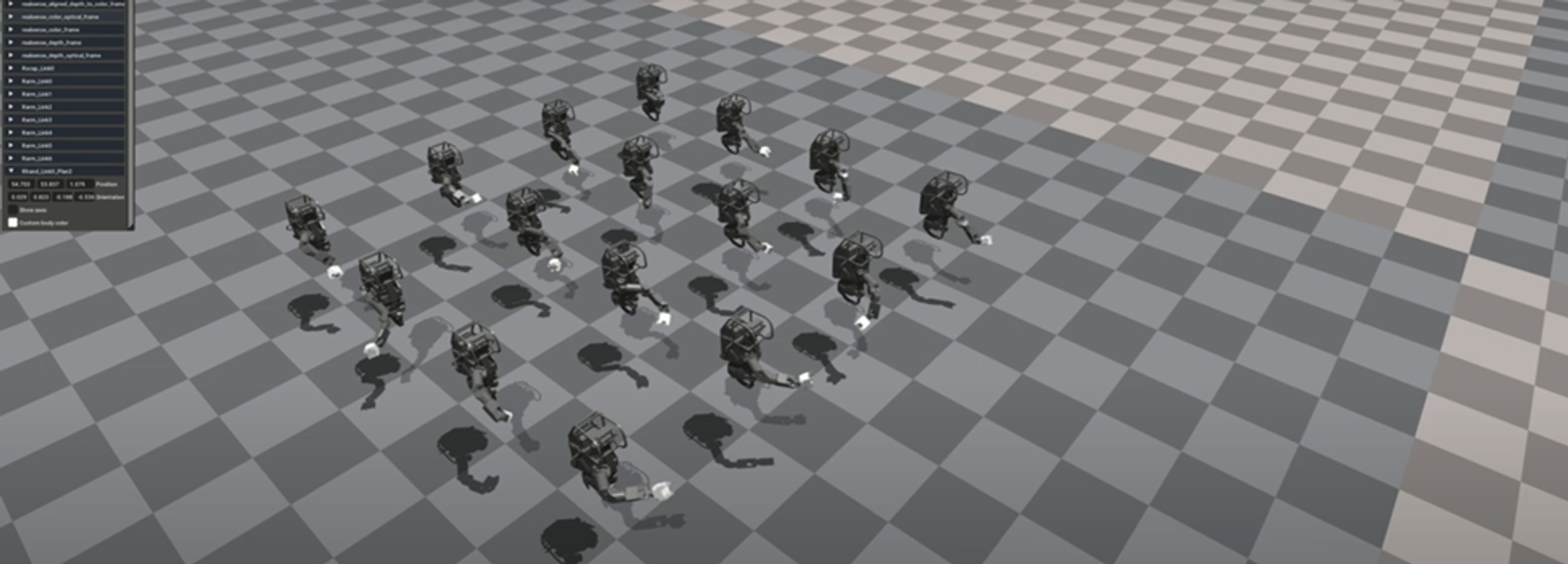
An illustration from the simulator while testing the task 4. The link white in color is the end-effector.
5. Reaching any given object in the Cartesian space from a random initial pose
In this task, objects have been added to the simulation environment that will be used as the goal for the end effector of the arm to reach. The position error: error in the 3D position coordinates of the arm’s end effector and the centre of the object is being minimized. The objects are spawned in random positions and orientations within the reachable workspace of the arm.
Observation Space: DoF positions and velocities, actions, goal pose coordinates: 3 position, 4 quaternion
Reward: Minimise position error, energy
Note: The grasp offset, i.e. the point of grasping used in the calculation and minimization of error is taken at a distance of 12.7 cm from the base of the end-effector link.
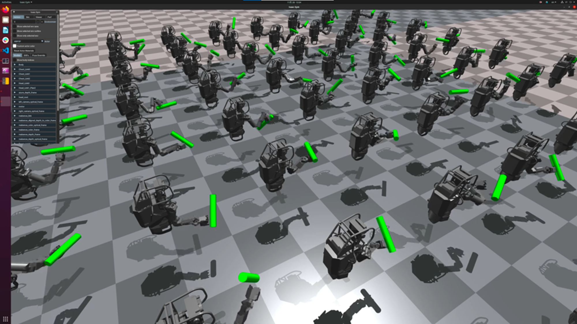
An illustration from the simulator while testing the task 5.
6. Reaching any given object in the Cartesian space from a random initial pose along with end effector orientation alignment
The task is a modification to the previous task 5 with an inclusion of the orientation alignment of the end effector with the object it is trying to reach.
Observation Space: DoF positions and velocities, actions, goal pose coordinates: 3 position, 4 quaternion, pose error
Reward: Minimise position error, energy
Note: The error for the orientation alignment is calculated by minimizing the angle between the local Z axis of the object and the local X axis of the end-effector.
An illustration from the simulator while testing the task 6.
The above tasks were simulated in Isaac Gym and trained using PPO with reward functions designed keeping in mind the respective intended goals as specified for each of the tasks above.
This post is licensed under CC BY 4.0 by the author.