SAUVC
This is a project on building an Autonomous Underwater Vehicle for the Singapore AUV Challenge. GitHub Repo
Building an Autonomous Underwater Vehicle. Check out the GitHub repository
We divided the project into three subsystems:
- Structures and Design Subsystem
- Electronics and Power Systems Subsystem
- Control and Navigation Subsystem
Structures and Design Subsystem
When it comes to Structures and Design subsystem their role is pretty straightforward, design and fabrication of different components required throughout the project. ROV frame, Canister/Enclosure, Propellers, etc. are designed and fabricated by this team.
Design and Fabrication:
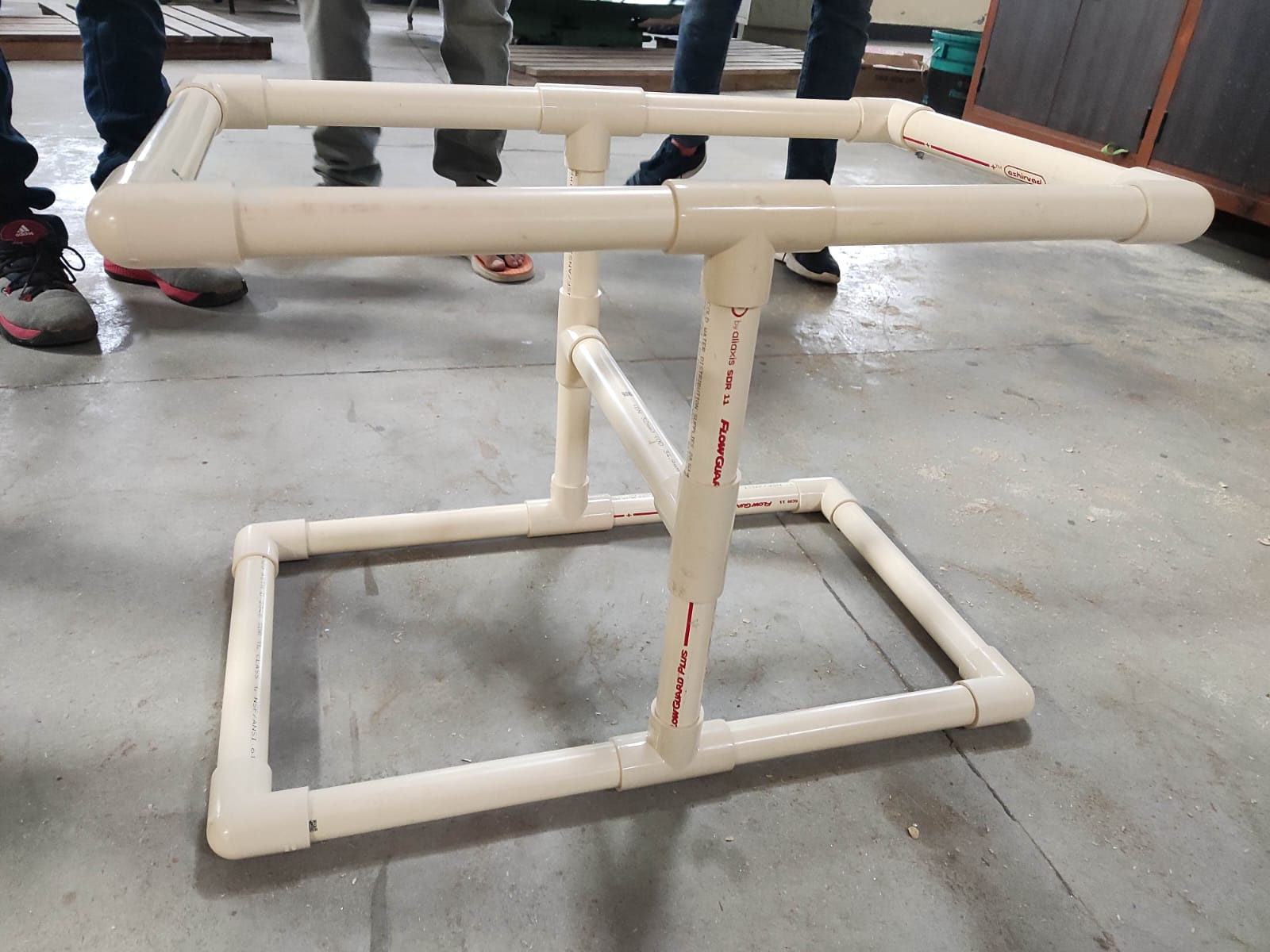
As part of our progress, we designed an ROV frame along with an AUV frame. We also fabricated the ROV frame using simple PVC pipes. We plan to finish the ROV first.
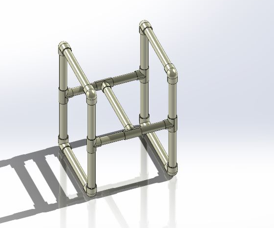
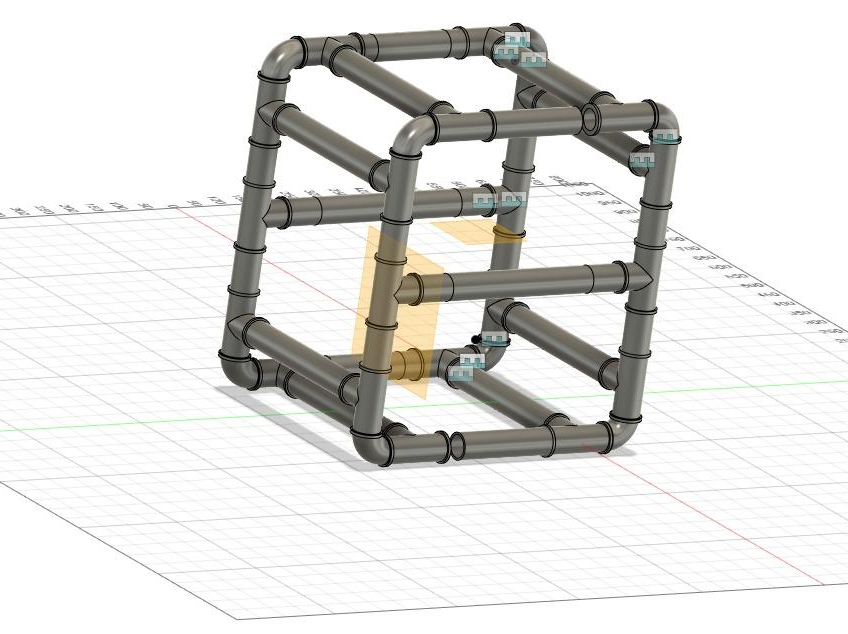
These CAD models will be utilized by the Control and Navigation team to run simulations in a Virtual environment created inside a physics engine called Gazebo.
The picture shows the assembled ROV Frame made from PVC Pipes.
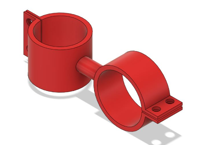
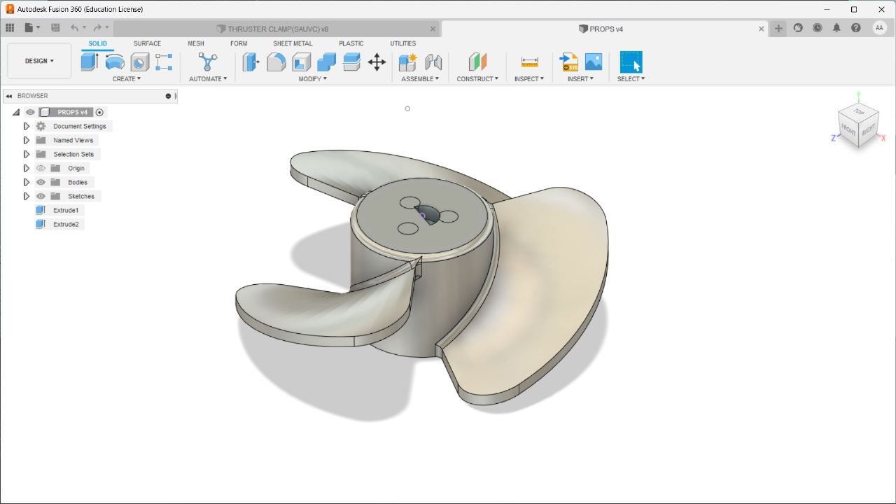
We also Designed the Thruster holder and Propeller to be used on motors.
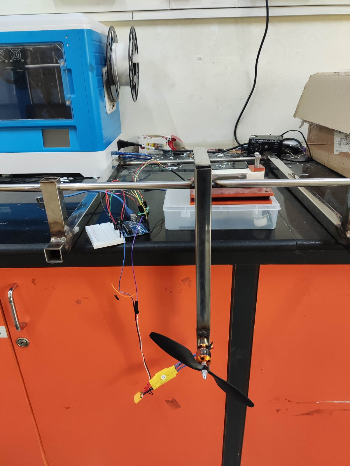
We also fabricated the Thruster Stand, an experimental setup to measure the Thrust.

COMSOL Analysis:
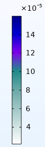
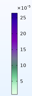
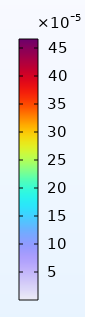
We also made a set of COMSOL Analysis on stress experienced by a Canister during its motion underwater for various shapes.
The analysis of stresses experienced by the canister is critical for canister structural design. It assists us in visualising and comprehending the motion of the canister and its response to stress and drag in a specific real-world situation. With the help of analysis, the geometry of the canisters can be optimised so that the body experiences the least amount of drag, which is our final aim.
Drag
Drag acting on a solid surface depends on multiple factors. The shape and size of the body affect the drag. The velocity of the flow, the viscosity and the angle of inclination of the flow are also all crucial factors affecting the drag. If we think of drag as aerodynamic friction, then the amount of drag depends on the surface roughness of the object; a smooth, waxed surface will produce less drag than a roughened surface. This effect is included in the drag coefficient. It also depends on the velocity of the fluid and body.
COMSOL Simulation
Our objective is to compare the drag forces, or the stress experienced on the bottom surface for a cuboidal and cylindrical canister with a hemispherical end. Solid Mechanics (solid) and Creeping Flow (SPF) were the physics modules chosen for this simulation. The Creeping Flow (spf) module was selected because the fluid flow (water) had an extremely low Reynolds number. Displacement and stresses can be computed using the Solid Mechanics (solid) module. The canister is made of Acrylic Plastic, and the fluid chosen for this simulation is water.
INITIAL VALUES:
Canister (Acrylic plastic): Initial velocity in x-direction = u_solid = 1.38 (m/s) Initial velocity in y-direction = v_solid = -0.1397 (m/s) Initial velocity in z-direction = w_solid = 0 (m/s)
Fluid (water): Initial velocity in x-direction = u_flow = 0 (m/s) Initial velocity in y-direction = v_flow = 0 (m/s) Initial velocity in z-direction = w_flow = 0 (m/s) Pressure = p = 101325 (kPa) Temperature = 293.15 (K)
GRAPHS:

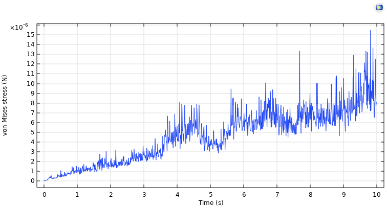
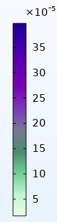
Graph1. Von Mises Stress on the square face of cuboidal canister vs. Time
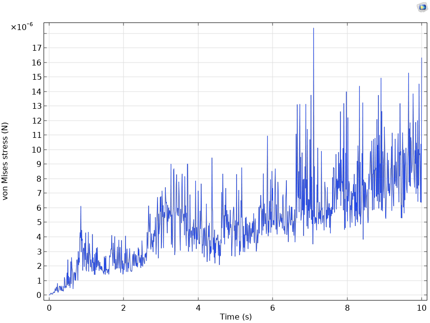
Graph2. Von Mises Stress on the Hemispherical surface of cylindrical canister vs. Time
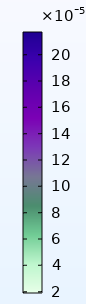
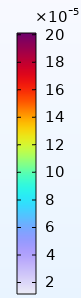
Graph3. Von Mises Stress on the bottom surface of cuboidal canister vs. Time
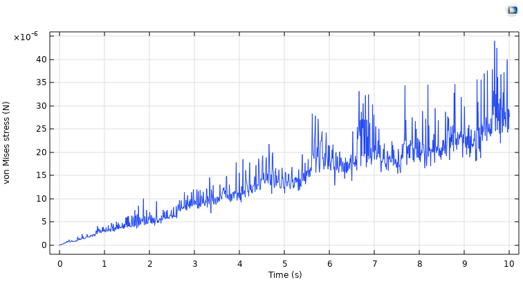
Graph4. Von Mises Stress on the bottom curved surface of cylindrical canister vs. Time
We observe that the cuboidal canister faces less Von Mises stress on the bottom surface. We can also see on comparing Graph.1 and Graph.2 that the Von Mises stress on the frontal face surfaces is significantly less in the case of cuboidal canister.
The involved Simulations are as follows:
Cuboidal face:

Cuboidal Bottom surface:

Cuboidal canister:

Cylinder Bottom surface:

Hemispherical surface:

Cylindrical canister:

Electronics and Power Systems Subsystem
The most important part of Power Systems in this project is the ‘Thruster’ and based on that, we will be able to decide the power supply. The electronic components that we are working on are used for purposes like maintaining the balance of the bot and environment sensing.
Different Motors as proposals for ROV thrusters:
BLDC Motors
We had planned to go with the BLDC motors as our ROV thrusters. BLDC motors are brushless and hence there is less loss of power. Also, the speed of the motors is higher, and they have been used by some other participants of SAUVC. We tested 2 BLDC motors - BR4114 and A2212.
Before diving into the motor specifications, it is very important to understand the Kv (not to be misunderstood with kilovolt) rating of a motor. The Kv rating of a BLDC motor is the ratio of the motor’s unloaded rpm to the peak voltage on the wires connected to the coils. It provides a basic idea of how much the motor RPM would be given an input voltage. A motor with higher Kv rating has few winds of thick wire that carry more amps at few volts and spin small props at high revolutions. On the other hand, a motor with a low Kv rating has more winds of thinner wire that will carry more volts at fewer amps and thus produce higher torque and swing larger propellers.
ESCs
An ESC (Electronic Speed Controller) is a device that is used to control and adjust the speed of BLDC motors. It is used in conjunction with the BLDC motors for various applications like in drones, etc. Therefore, the required specifications of the ESC we need to use are highly dependent on the BLDC motor we choose for our job.
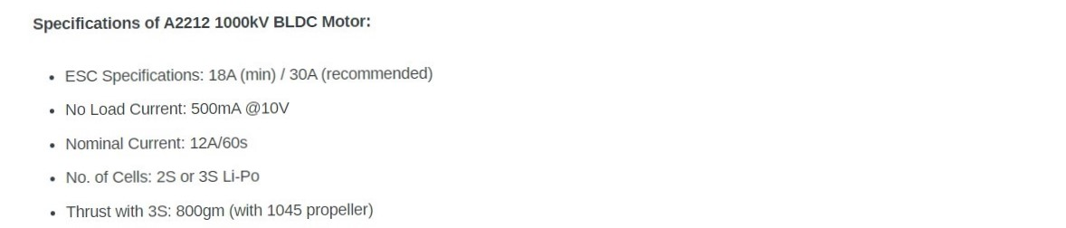
a) A2212:
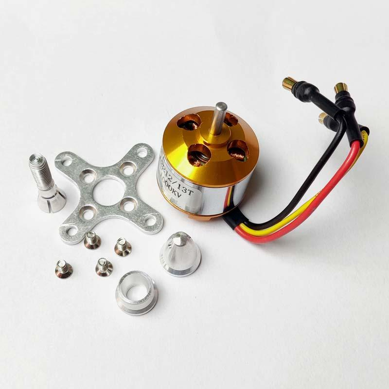
The A2212 motor is a 3-phase outrunner-type BLDC motor that is commonly used in drones and other multirotor applications. Its specifications are as follows:
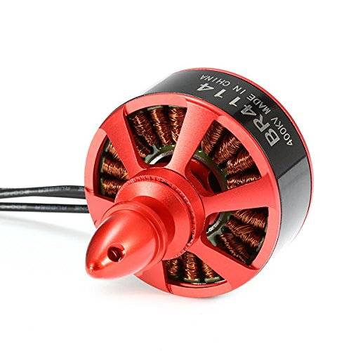
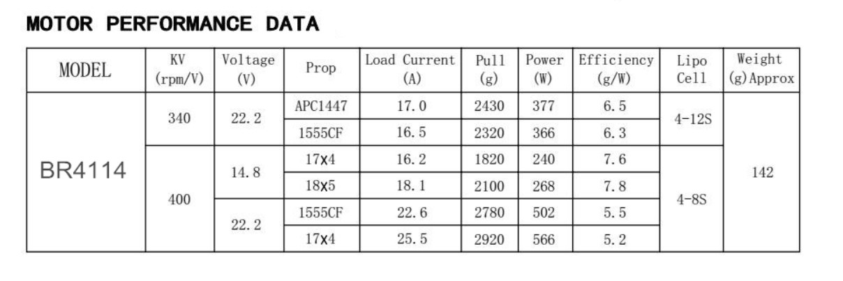
b) BR4114:
The BR4114 is typically used in multirotor applications just like the A2212. But since it has a lower Kv rating as mentioned below, it can be used in applications where larger torques are needed.
We tested the motors using the 4S LIPO battery and controlled the speed using a 30A ESC. The specifications of BR4114 are as follows:
The main issues encountered with the BLDC motor were:
- The ratio of thrust output given to the input power taken was very poor and hence inefficient.
- We need to make the BLDC motors waterproof. They may work in fresh waters but if the water contains salt, it may corrode, and the efficiency may reduce drastically. Instead, we decided to use a Bilge pump which can be placed in water directly because they are sealed properly.
Bilge pumps
Bilge pumps are pretty solid alternatives to the BLDC motors since they are already sealed and waterproof. We tested the bilge pumps using the variable DC power supply.
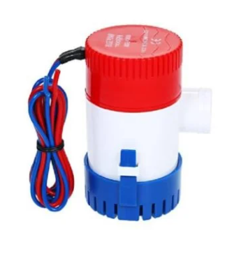
It operates at a 12V DC power supply and pushes the water out at the rate of 750GPH (Gallons per hour flow rate). Specifications of the Bilge pump: Voltage: 12.0 V DC Current: 3.0 A Flow rate: 750 GPH We can clearly see that the power requirement of the bilge pump is less than BLDC motors and the water that is being pushed out is relatively high.
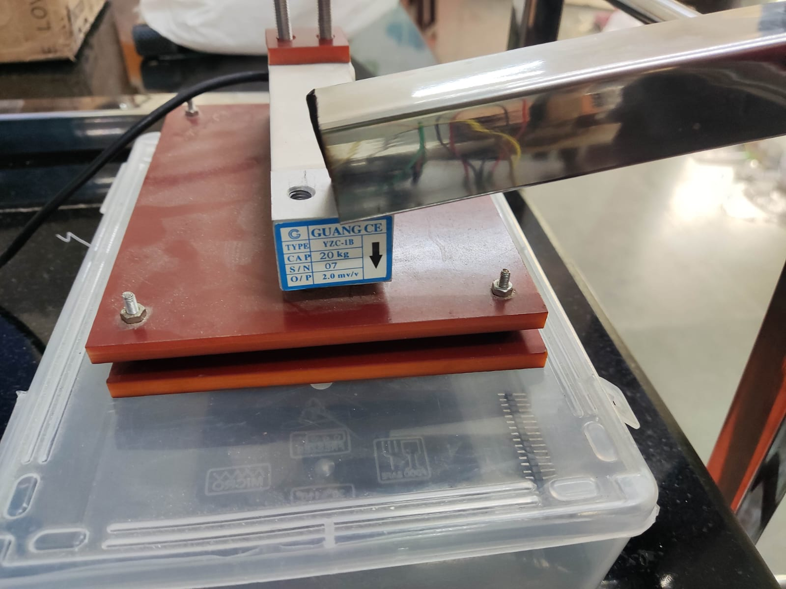
Thruster Stand
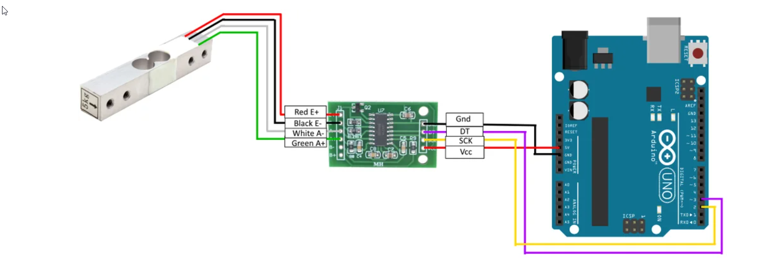
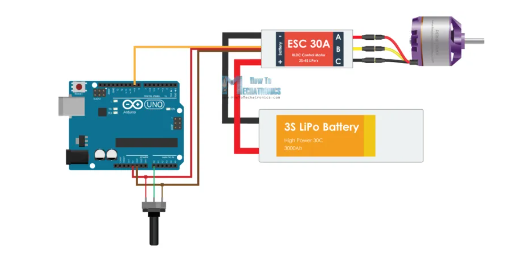
Our experimental setup involves the following two circuits joined together. Circuit 1 consists of a Load Cell connected to Arduino through an Amplifier (HX711). This setup helps us to measure the force exerted by any object within the load cell’s range, in our case, 20kg. Circuit 2 is used to control the BLDC (Brush-Less DC) Motor. For our case, we used a BLDC as a thruster. The circuit should be changed somewhat if we use other motors like DC motors.
Circuit 1
Circuit 2
Before the Impact of the L–Shaped Rod After the Impact of the L–Shaped Rod

BLDC mounted to the thruster stand

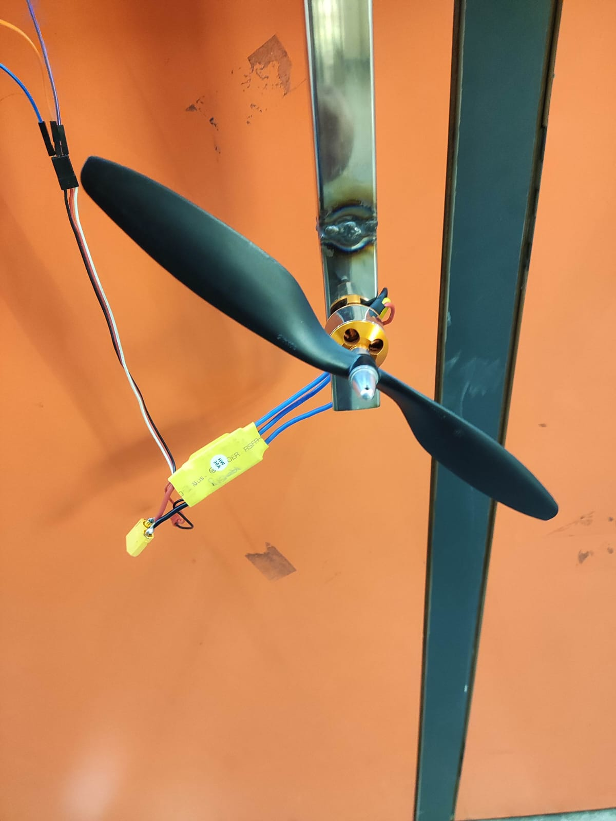
The L–Shaped rod has one degree of freedom, rotational motion along the axis passing the intersection. Due to this, when the thruster is powered, the thrust generated will rotate it. This rotation will make it have an impact on the load cell.
The reading that we get from the Load cell will be that of the normal reaction of the L-shaped rod and load cell. To get the thrust value, we must balance the torques about the point of intersection, i.e. from the axis of rotation.
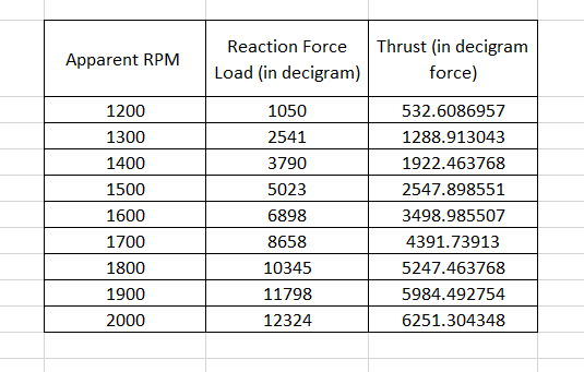
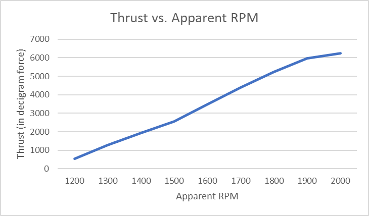
Here for testing purposes, we measured the Thrust generated by a thruster used in Drones. Then we made a plot of these values with an alias of RPM which we gave through the code called apparent RPM, where 1000 means minimum RPM and 2000 means maximum RPM.
Video: Working Video
Circuit diagram for the ROV
a) For Off-board power supply:
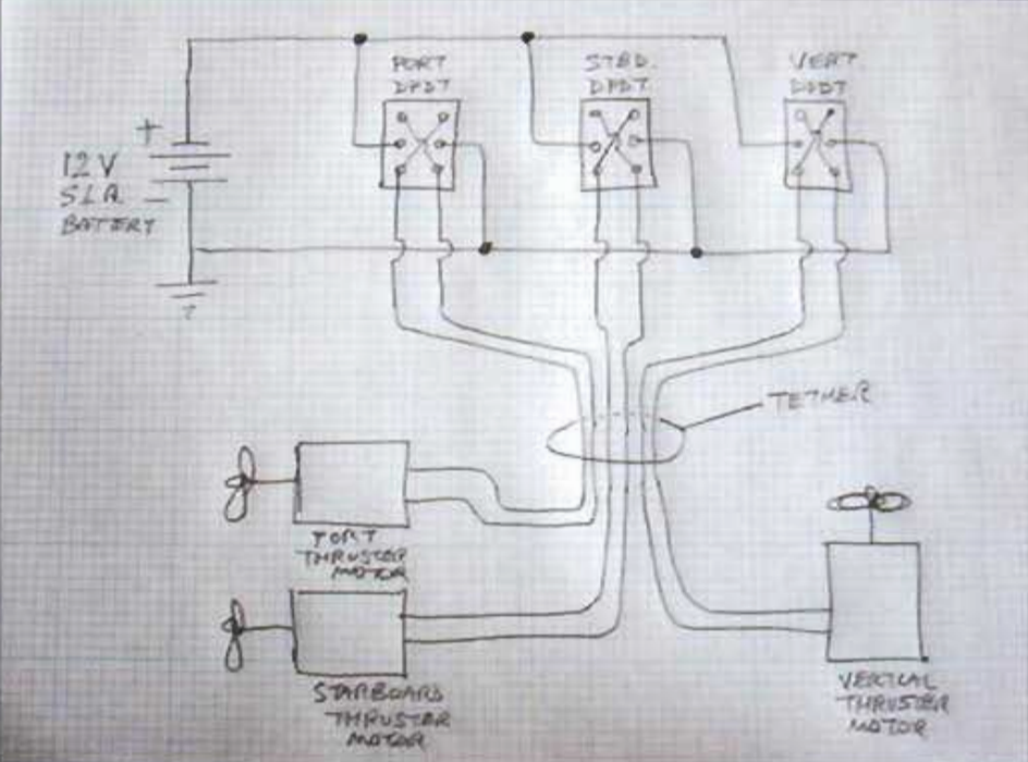
• This is a three-thruster arrangement: one for heave motion and the remaining two for surge and yaw motions(3 DOF). • The DPDT switches are used for: ◦ Switching the motors ON/OFF and ◦ Changing the sense of rotation of the motor. • The tether used here is well insulated and it consists of an ethernet cable with six lines(two for each motor) that control the working of the motor.
For the above method to work when we will use our campus swimming pool for testing, we should probably use batteries as there is no power plug available to use an SMPS. We are yet to decide if we are going to use this method of power supply being away from the bot. The following is the plan if we use the on-board variant.
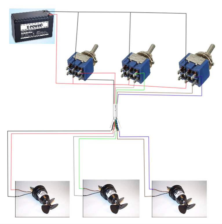
b) For On-board power supply:
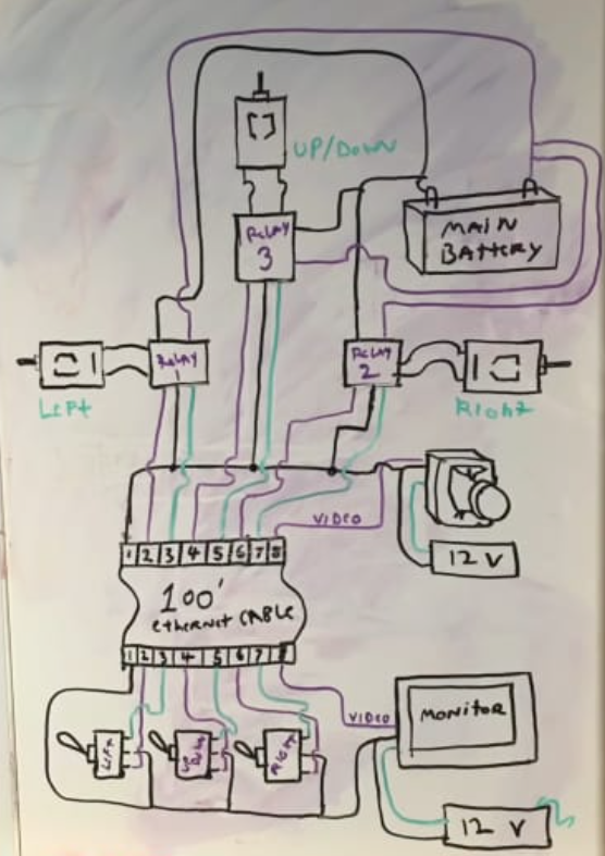
• Here, since the power supply is on the bot, we should use a different circuitry. The lower part of the above schematic is the operating/controlling end while the top part(w.r.t the tether) is on the ROV. • The user will be using DPDT switches as in the previous case but here, the power supply on the bot is connected to the thrusters through ‘Relays’ which provide the power to them based on the input of the operator. Also, there is power supply at the user’s end. • For the ROV, we are not working on the Camera part, so from the above schematic, it should be ignored.
Implementation of Control System
PID Controller with no nonlinearity compensation:
x, y, z: Linear positions in world frame phi, theta, psi: Angular positions in world frame


PID Controller with nonlinearity compensation:
x, y, z: Linear positions in world frame phi, theta, psi: Angular positions in world frame
u, v, w: linear velocities in body frame p, q, r: angular velocities in body frame
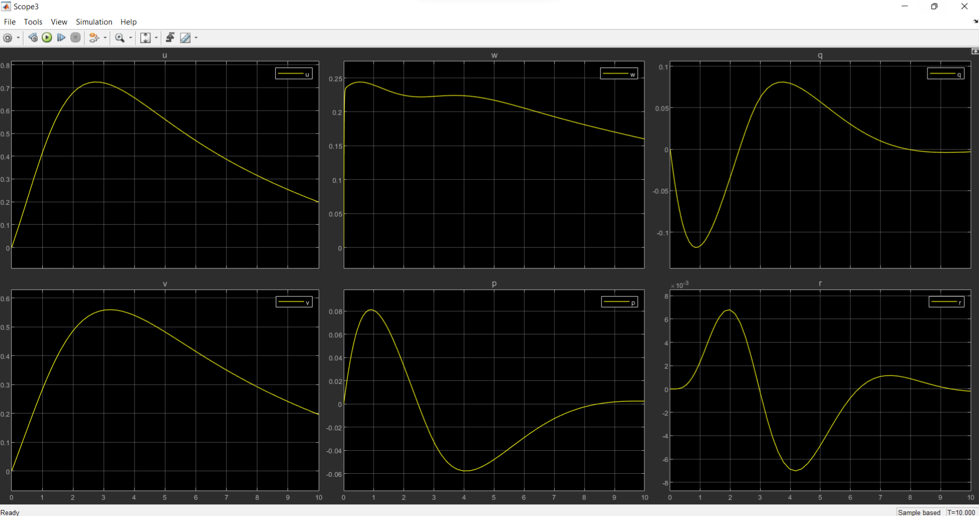
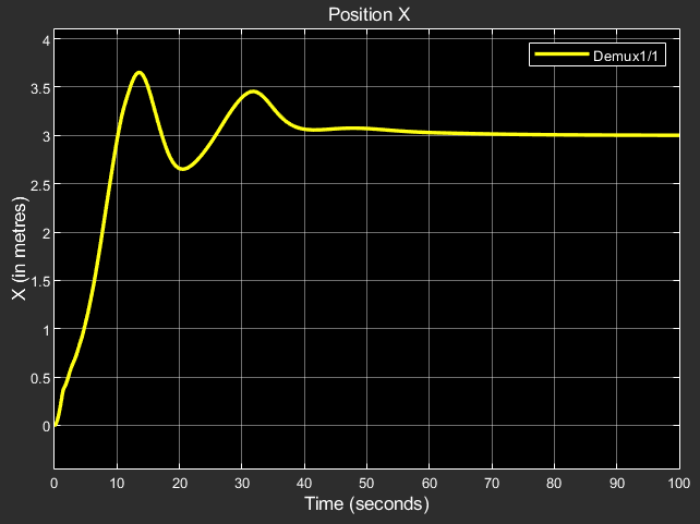
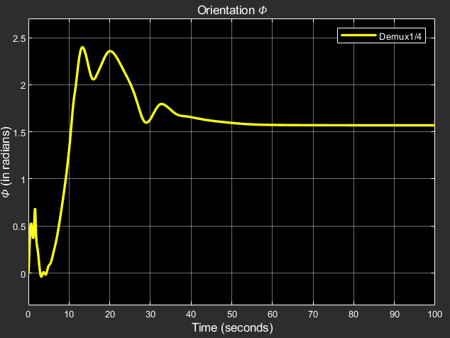
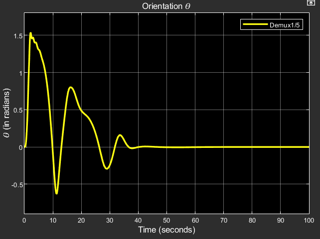
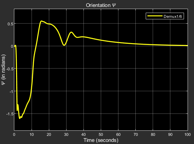
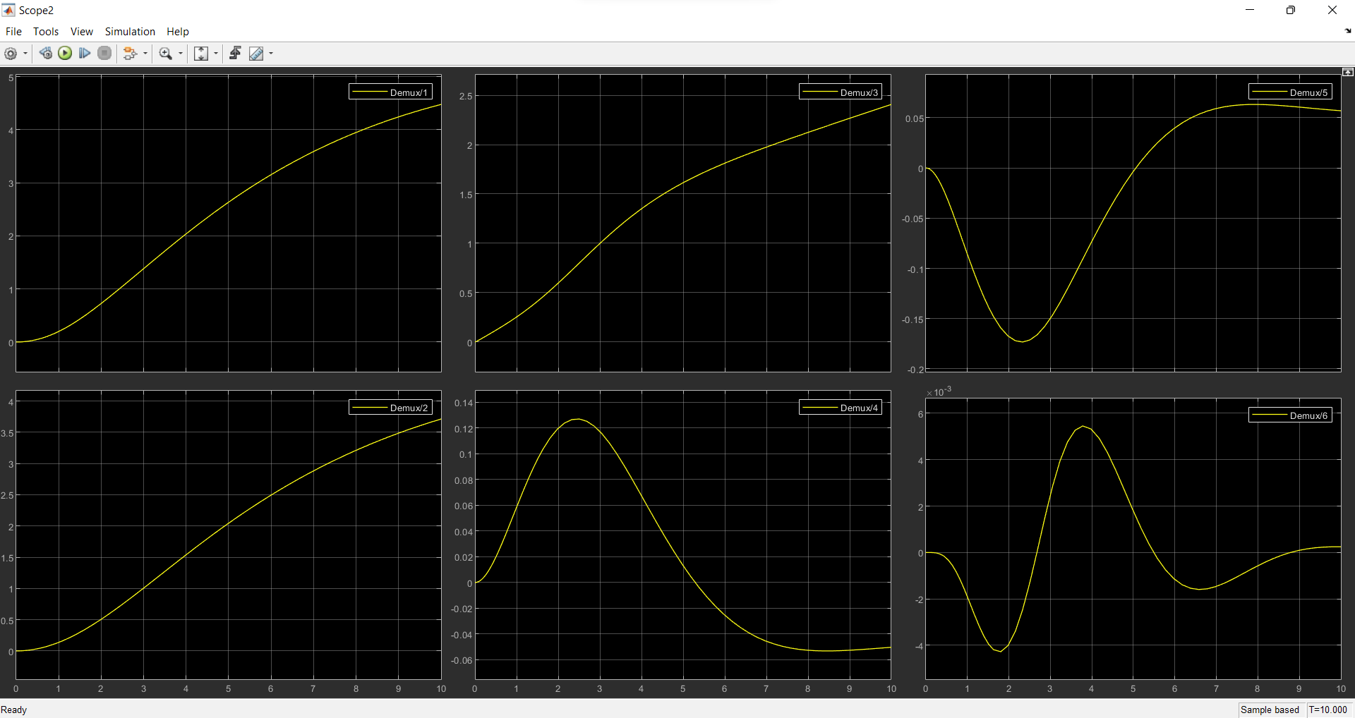
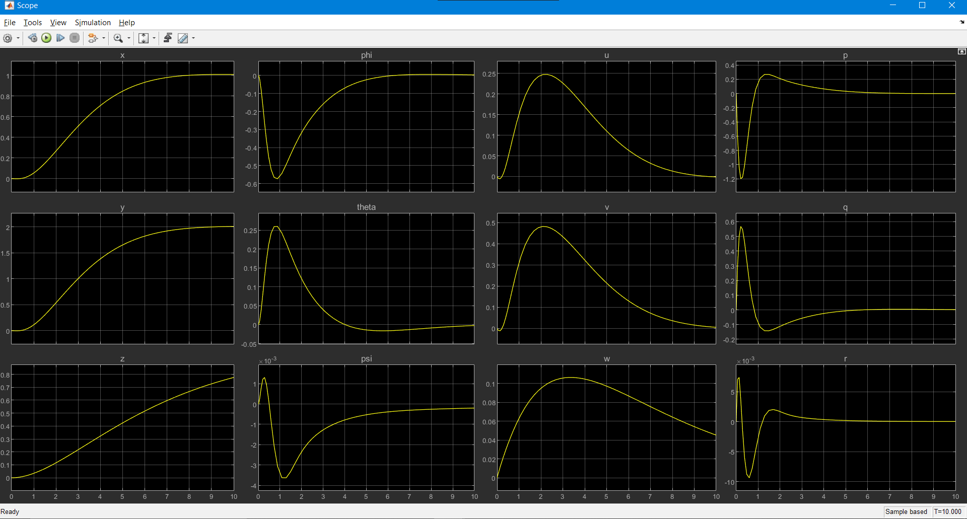
LQR Controller:
Results that we obtained: x, y, z: Linear positions in world frame phi, theta, psi: Angular positions in world frame u, v, w: linear velocities in body frame p, q, r: angular velocities in body frame
A Comprehensive report on the control system for the AUV can be found here: Position and Velocity Control of a 6-DOF AUV
Control and Navigation Subsystem
Simulations
Simulation is an important aspect of building an Autonomous Underwater Vehicle (AUV). It allows the team to test and validate the robot’s design and performance in a controlled environment before deploying it in the actual competition. Simulations also enable us to identify and troubleshoot potential issues before they occur in the field, which can save valuable time and resources.
It helps us test various aspects of the robot’s design, such as its hydrodynamics, control algorithms, and sensor systems. By simulating the robot’s movement and behavior in different scenarios and environments, we can optimize its design for maximum performance.
Additionally, simulation can be used to test the robot’s autonomy and decision-making capabilities. The simulated robot can be programmed to respond to different situations and tasks, such as obstacle avoidance, path planning, and target tracking. This can help the team to build a more robust and capable robot, which can improve its chances of success in the competition.
All the simulations were carried out on Gazebo using Robot Operating System (ROS). The following were the components of the simulation/testing process:
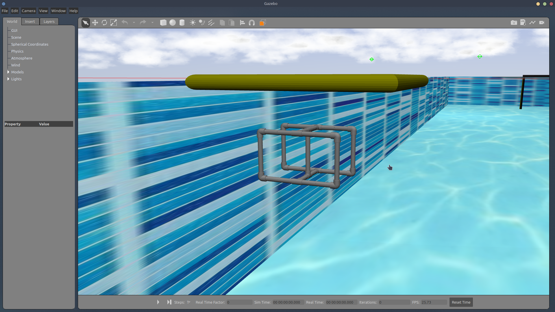
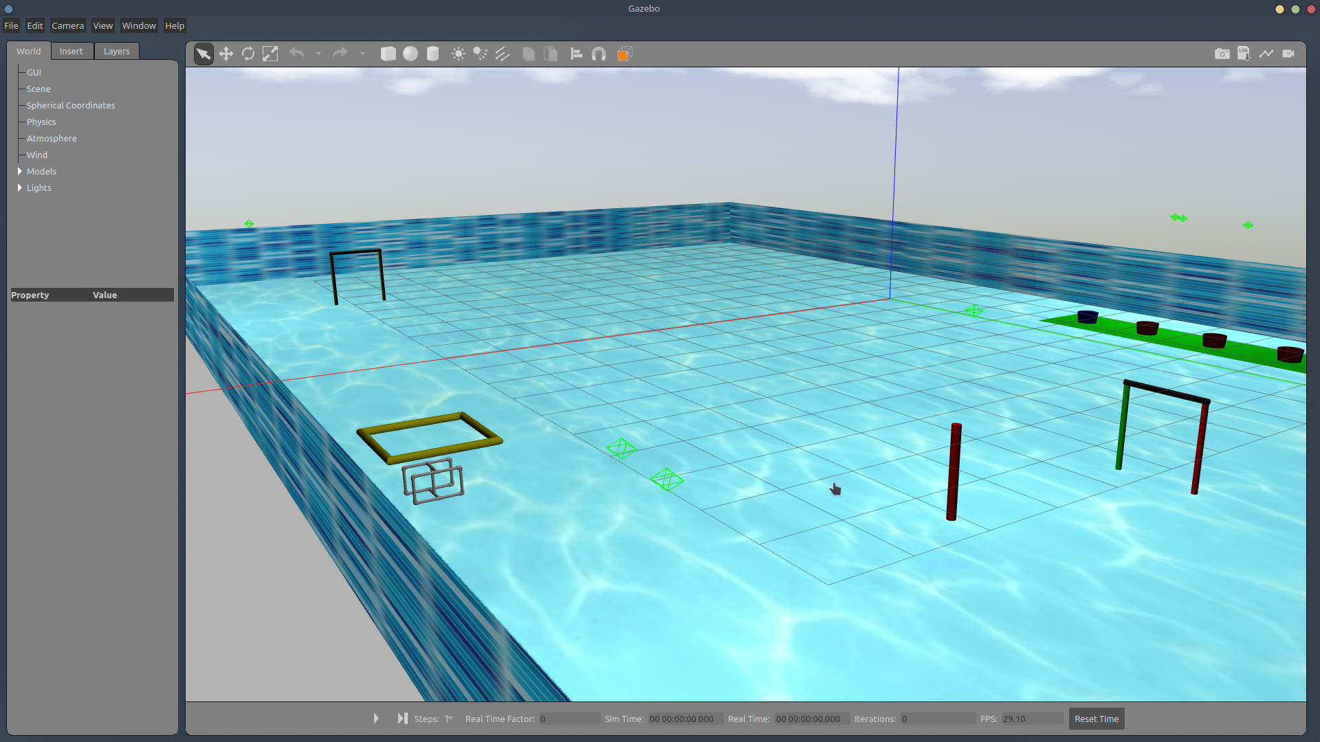
Environment - The initial environment consisted of an open ocean with objects such as a shipwreck. This environment was not enough to satisfy the simulations needed, so a pool environment called sauvc_pool which contained accurate information about the size of the pool as well as the obstacles and tasks inside the pool was implemented.
Bluerov2(ffg) - The bot we chose to simulate was the bluerov2 from Bluerobotics, as it consisted of a 6-thruster design, and its thrusters would give us an accurate idea of our own thrusters.
Bluerov in pool - The bot was integrated into the sauvc_pool environment, where it could freely interact with the tasks and obstacles. Since it was operated in ROV (Remotely Operated Vehicle) mode and not AUV mode, the bot had to be controlled with keyboard input. Simulation Video: https://drive.google.com/file/d/1jb7FUMZcOFuTcBESvxL-OGILuCvJh7Xp/view?usp=sharing
6 thruster AUV in pool - Bluerov2 has 6 thrusters, but in our tests, we need to simulate the results for an AUV having anywhere from 1 to 6 thrusters and testing its DOF’s, thrust values, etc. For this, the bluerov2’s URDF files were tweaked to include/exclude thrusters as well as specify the directions they were pointed in. Simulation Video: https://drive.google.com/file/d/1xc2mSkLJA_p5KI65yUyRHvm-LtWhhFbn/view?usp=sharing
ROV in pool - After this, we imported the STL file of our own SAUVC entry into Gazebo for simulation in place of the bluerov2. The file followed the same format as that of the bluerov2 so that the thruster locations, thrust values, as well as ROV operation is possible for our bot the same way as the bluerov2.
Object Detection
Object detection is a computer technology related to computer vision and image processing that deals with detecting instances of semantic objects of a certain class in digital images and videos. One popular algorithm for object detection is YOLO (You Only Look Once). YOLO uses a single neural network to predict bounding boxes and class probabilities directly from full images in one evaluation. It’s become popular in real-time object detection because of its speed, as well as its ability to detect a large number of object classes.
Using YOLO for object detection in an underwater environment, however, is a challenging task. The lighting conditions, turbidity, and low visibility can affect the performance of the algorithm. In addition, underwater images may have different characteristics than images taken in an above-water environment, such as color distortion, refraction, and reflection. To overcome these challenges, image pre-processing and training the model on a dataset of underwater images is crucial. This dataset should include a variety of underwater scenarios, lighting conditions, and different types of objects.
In the context of the Singapore Autonomous Underwater Vehicle Challenge (SAUVC), YOLO can be used to detect and classify various objects in the underwater environment. This can help to improve the navigation and control of the autonomous underwater vehicle (AUV). For example, YOLO can be used to detect obstacles and map the environment, which can be used to plan a safe and efficient path for the AUV to follow. YOLO can also be used to identify targets of interest, such as underwater structures or objects of a specific class. Furthermore, object detection information can be used to trigger specific actions or behaviors of the AUV, such as obstacle avoidance, and capturing images or samples of a specific object.
In the SAUVC competition, the vehicle is required to navigate in an unknown and unstructured environment. The object detection algorithm can be used for mission planning and localization and can help the vehicle perform more complex tasks, such as search and recovery.
The following video shows a real-time demonstration of YOLO: https://drive.google.com/file/d/13KlP3ML55CJQzNvX7uuXz6ovnkqePeDQ/view?usp=sharing
Depth Estimation
Depth estimation forms an important aspect of the SAUVC competition for several reasons.
Firstly, depth estimation allows the robot to determine its own position in the underwater environment. This information can be used for localization, navigation, and obstacle avoidance. For example, the robot can use depth information to plan its path and avoid areas that are too deep or shallow. Secondly, depth estimation can also be used to detect and avoid obstacles by comparing the estimated depth of an object with the expected depth of the environment. This can be used to improve the safety of the robot and prevent collisions.
Thirdly, depth estimation, together with object detection techniques such as YOLO, can be used to identify and track targets of interest in the underwater environment, such as specific structures or objects. The robot can use depth information to determine the position of the target and navigate toward it.
Lastly, depth estimation can also be used for scientific research, as it can aid in generating 3D maps of the underwater environment and make measurements of the characteristics of the water column like salinity, temperature, etc.
The common ways to estimate the depth are:
- Using a Depth Sensor: This is a sensor specifically designed to measure the distance to an object. It can be an active sensor like a sonar, or a passive sensor like a stereo camera.
- Triangulation: it uses information from multiple sensors, such as cameras and lasers, to determine the distance to an object based on its apparent size in the sensor’s field of view.
- Structure from motion: it uses multiple images of an object taken from different perspectives to estimate its depth based on the apparent motion of the object in the images.
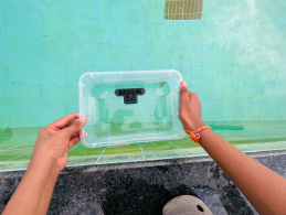
For the purpose of this competition, depth estimation is performed using the OAK-D depth camera. The depth camera calibrated in the air cannot be used for performing underwater experiments due to differences in disparities caused by the refraction of light. As a result, it needs to be calibrated underwater and then used for depth estimation.
The setup to perform underwater depth measurement involves placing the OAK-D depth camera in a transparent container and holding it inside water partially submerged, as shown in the images below. The entire setup and all the experiments were performed in the swimming pool.

Camera Calibration:
The camera is calibrated using a charuco board, in a process very similar to calibrating using the Zhang Zhengyou technique. The charuco board is printed onto a flat surface, and 13 different images are captured in different orientations. Once the camera calibration is complete, we obtain the distortion coefficients, intrinsic parameters, extrinsic parameters, and the stereo rectification data of the camera.
Depth Estimation:
The disparity and depth can then be obtained from the stereo camera pair. By performing experiments underwater, the depth values and the disparity map are obtained as follows -

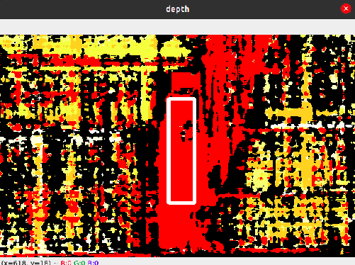

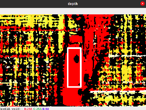


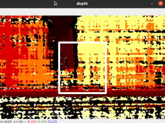
From the above images, we see that as the bottle is placed farther away from the depth camera setup, the value of the depth increases, and the disparity map changes accordingly. From the experiments performed above, we find that the depth camera can measure a depth of up to 1m (~3ft) underwater.
Camera Localization:
Using the extrinsic parameters of the depth camera, which were obtained earlier during calibration, the position of the depth camera can be estimated.

The entire camera setup needs to be enclosed in a waterproof canister. Improving the lighting conditions using subsea LED lights would enable us to measure larger depths.
Acoustic Localization
Localization is required to complete the target acquisition and re-acquisition task in the challenge. The pingers fitted to the drums act as an acoustic source. A 2/3/4 acoustic sensor setup can be used for localization. There are different localization techniques, such as received signal strength indication (RSSI), angle of arrival (AOA), time difference of arrival (TDOA), and time of arrival (TOA), of which different methods are used in various applications. The angle of arrival estimates is found by using TDOA, and the far-field approach is followed for simplicity.
Time difference of arrival estimation:
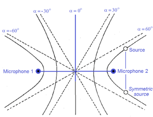
- We get a hyperbola with two possible locations with two hydrophones, and with four hydrophones, it is easier to find the location of the source.
- The time difference between the two microphones is computed and used in estimating the position of the acoustic source.
Finding the time difference:
The following methods are widely used, with each having its pros and cons:
- Normalized frequency-based TDOA: This method can be used when the source is of a single frequency(and the value is known). We convert the obtained signals into the frequency domain and use the phase difference to find the time difference, and this method is prone to noise.
- GCC-PHAT: This is based on the GCC algorithm. In order to compute the TDOA between the reference channel and any other channel for any given segment, it is usual to estimate it as the delay that causes the cross-correlation between the two signal segments to be maximum. This method is less prone to noise but is computationally expensive.
- Hilbert transformation: This method works well for narrow-band signals and can be simplified using FFT to reduce computational costs and gives good results when compared to cross-correlation methods.